How Infrastucture as Code Works

Some of the most powerful tools in technology take the form of new abstractions, taking some new arbitrarily complex task and simplifying it to a set of inputs and outputs. Google, for example, simplifies the task of searching the entire internet for content down to a simple interface: give us a text query, we’ll give you some good results. Powerful programming frameworks give developers the ability to write application behavior that would otherwise be entirely unfeasible; Spark is a good example. Abstractions are powerful because they do not just provide the ability to complete some new task, but act as a building block that can be used as a component of another layer of abstraction on top of them.

One of the most powerful categories of abstraction is in cloud infrastructure, meaning a set of services provided via API and often other means to create, manage, and destroy infrastructure. AWS, Azure, and GCP are three of the most prominent providers in these areas, and while their approaches differ in myriad ways, they all also provide a similar set of core abstractions such as on-demand servers and object storage buckets. Modern technology companies (and many non-strictly-technology companies) may maintain hundreds or thousands of these components at minimum, many of which might have dependencies between one another. The ability to scale systems by adding more and more components from the set of services these cloud providers offer is part of what makes them powerful, but it can also introduce massive operational cost and complexity to internal operators of these systems. The category of software that effectively manages an individual or organization’s resources within cloud or other API providers is still very new, and some of the most powerful tools I’ve found within it have been infrastructure-as-code (infra-as-code) tools. If you aren’t familiar with infra-as-code at all it’s work checking out the Terraform introduction page; Terraform is the first tool I’m aware of in this category and was first released in July 2014. Another notable tool in the space is Pulumi, which first shipped in May 2018.

I was fascinated by infra-as-code tools since my first exposure to them in 2017, and about a year ago I set out to learn everything I could about how they worked by building one. The result was a project I call statey. In creating statey, I first tried to fully conceptualize the underlying data model and algorithm that infra-as-code tools were built on. I started to form a clear model about how the internals of these tools operate. What I present here is a simple model that demonstrates how infra-as-code tools turn a declarative configuration and a saved state into a plan to transform your managed infrastructure from its current state to your configured one. One notable thing, however, is that the model doesn’t rely on anything having to do with cloud infrastructure or APIs at all—it’s entirely constructed based on mathematical concepts. To understand the connection between this model and the interface these tools provide, I’ll quickly explain the core similarity between all infra-as-code tools: resources.

Resources

Every infrastructure-as-code tool or framework on the market today is centered around the concept of resources. A resource translates to something in the real world, like an AWS server—it exists, you’re being charged for it, and someone might be in trouble if you can’t maintain access to it. Implementationally it generally maps to some sort of stateful API, or something you can create, update, and delete—that’s a general description, but conceptually it really is that general. How resources work is that you provide the tool with some configuration—for an AWS EC2 Instance (server) this might be the size, the machine image to use, and some network configuration for example. That configuration is declarative—meaning the user does not tell Terraform or Pulumi what specific operations to execute, only the desired end state. This is an example of a terraform EC2 Instance configuration:

resource "aws_instance" "my_server" {
 instance_type = "t2.micro"
 ami = "ami-0f400b8037c2bef6c"
}

And, incidentally, the same using pulumi and statey respectively (note that in all cases, the configurations look more or less the same):

import pulumi
import pulumi_aws as aws

web = aws.ec2.Instance(
   "web",
   ami="ami-0f400b8037c2bef6c",
   instance_type="t2.micro"
)

from statey.ext.pulumi.providers import aws

web = aws.ec2.Instance(
   ami="ami-0f400b8037c2bef6c",
   instanceType="t2.micro"
)

Resources can also rely on one another (just so long as none of those dependencies form a cycle), and all of this configuration can be updated incrementally as you go, as well as torn down at any moment. For example: a server might rely on various network resources it is attached to, like a security group or subnet in AWS parlance. Whenever Terraform or Pulumi are given a new configuration, they use that and the existing resource state to form a “plan” that takes all dependencies into account and will reach the desired state with the minimum number of changes required to each resource (theoretically).

While I won’t spend too long going deep into all of the possible things that can be done with resources in these tools, if you aren’t familiar with them I encourage you to read Pulumi’s Programming Model page or the Terraform Configuration Language Documentation, both describe how resources can depend on one another and how different dependencies can be configured for the relevant tool. A couple of additional resources for further reading would be Pulumi’s Architecture and Concepts page and Terraform’s How Terraform Works page.

What every infrastructure-as-code tool has in common

For the purposes of establishing a model for thinking about how infrastructure as code tools work, rather than focus too much on how resources work in particular tools I’ll zoom out and attempt to define what all of these tools are doing more abstractly.

One thing resources have in common in any infrastructure-as-code tool is they fit the mathematical definition of a finite state machine. A finite state machine consists of a few things: a finite set of possible states, a finite set of possible inputs, and a finite set of transitions. There is one transition for each pair of an input and a state that gives the new state of the machine. It is a bit simpler to see visually—the following shows a fairly typical diagram showing the transitions of a simple finite state machine. In this case, there are two states: A, and A’. There are two inputs: E0 and E1. The input E0 maps any state to A, and the input E1 maps any state to A’. In the real world resources would have a massive number of potential states, but this simple example illustrates the same logic on a small scale.

The declarative configuration that is provided to Terraform, Pulumi, or other infrastructure as code tools can be described as a set of finite state machines that depend on one another. In fact, for those with a little bit of familiarity with graph theory we can describe this graph of dependencies as a directed acyclic graph, commonly abbreviated as DAG. For those without any, the concept is intuitive: this just means that none of the dependencies in the configuration form a cycle with one another; a simple example of one such configuration with some resources named A, B, C, D, and E would be:

In the declarative configuration given to the infrastructure-as-code tool, the configuration of A depends on the states of B and C, and the configuration of C depends on the states of D and E.

Now, the interesting question is how we would actually go about creating the set of resources with this configuration. Since the configuration of A depends on the state of B, certainly we cannot create A until B has already been created—otherwise we wouldn’t fully know the correct configuration values! The same goes for any of the dependencies displayed in the diagram above. To formalize that a bit more, it is useful to visualize what these transitions would look like in the same diagram:

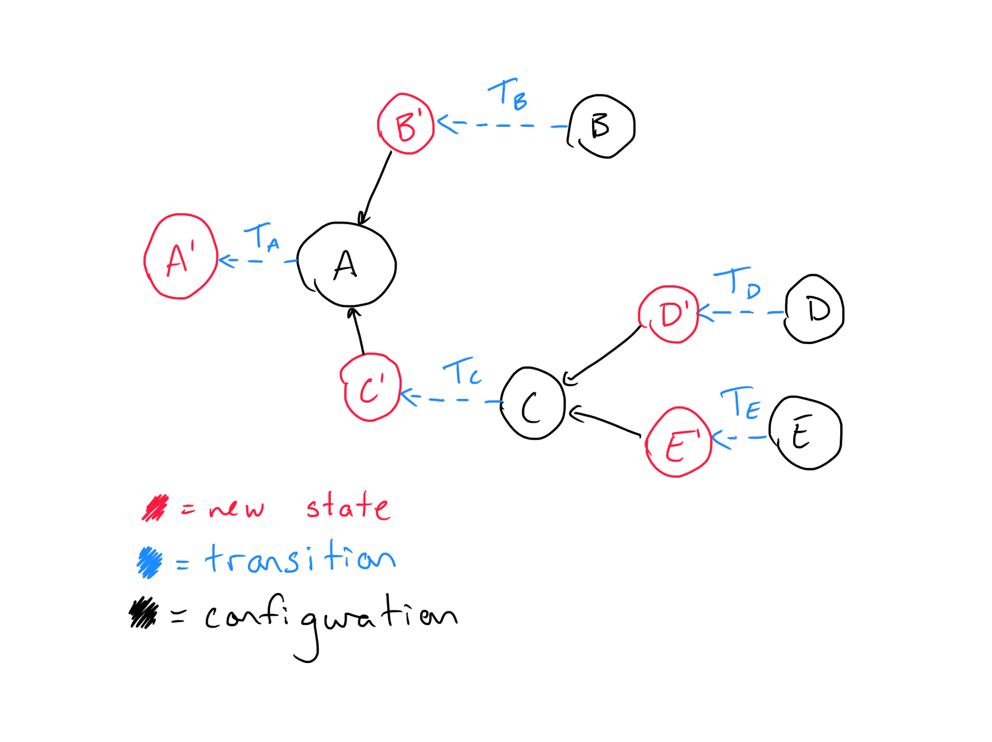
Here each node has been expanded to show that its “in” edges imply that it depends on the “after transition” states of other resources and its “out” edges imply that another resource’s configuration depends on its output state. In using this visualization, it is clear that there is some implied dependency between the transitions. If we remove the configuration and “new state” nodes while keeping all the same dependencies, we are left with a graph showing us how transitions for each resource depend on one another:

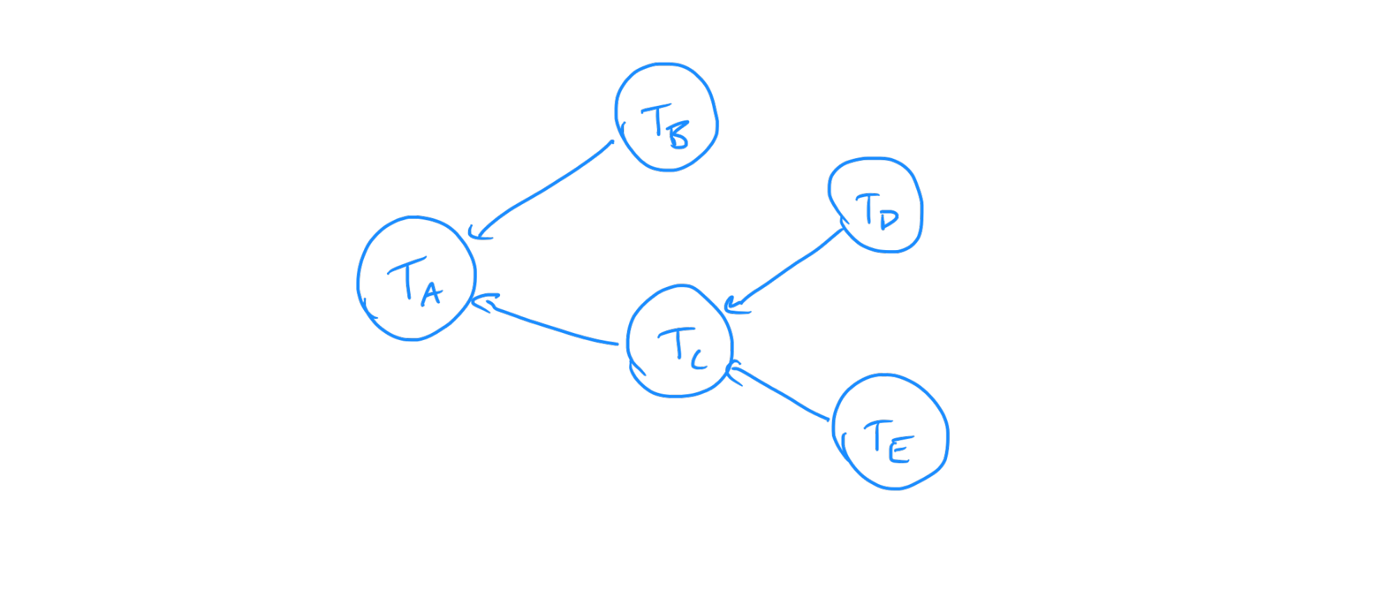
This looks familiar—it is the same as the dependency diagram for the initial configurations. In the simple case when resources are being created from nothing, the resulting task graph is exactly the same as the graph showing dependencies between the resources’ configurations. However, as soon as we want to update the configuration, the task becomes a more complex.

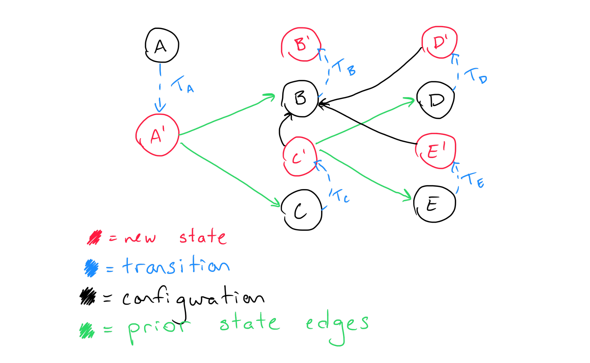
This exercise gets interesting when we reason through what has to happen given some new configuration, with new dependencies. As an example, assume we have a new configuration that we’d like to migrate our state to that looks like this:

Now instead of the previous dependencies B’s configuration depends on the states of C, D, and E. We’re attempting to apply this configuration immediately after the previous one has been applied successfully. It is no longer trivial to determine what order we have to update each of these nodes’ configurations in: if one resource depends on another in the previous configuration, the resource it depends on should not be changed until it is no longer depended on—consider a security group in AWS. AWS Instances can be bound to security groups, which would translate to a dependency in the configuration between the two. If we tried to delete the security group before the instance no longer depended on it, the operation would fail and manual intervention would be required. Considering how common this sort of case is, if infrastructure-as-code tools didn’t take this into account they would not be very useful and would often fail to execute their operations successfully.

Because we need to take these dependencies into account, we need to build the diagram including both states and transitions required to migrate to the desired configuration taking the previous state’s dependencies into account. The way we do this is relatively simple: we include them as edges alongside the edges implied by the configuration, but we reverse them:

If we reduce this diagram down to the transitions while retaining the dependencies, we get the following:

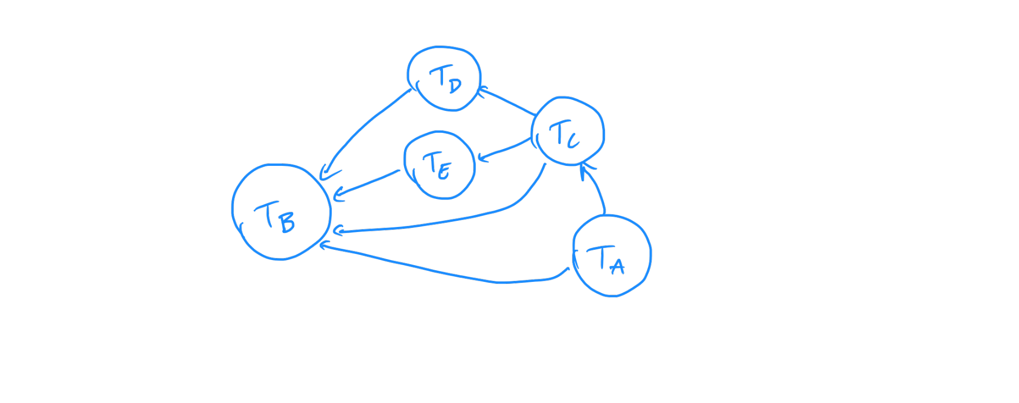
This tells us what order each of the transitions need to be executed in order to properly respect both the old and new configuration dependencies.

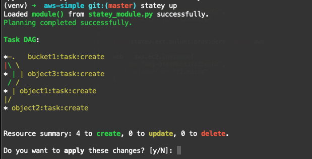
This general technique can be used to determine how to migrate between any two configurations, incrementally applying changes as and where required. There are a couple of other important cases and nuances to consider if one wants to go write a tool that does this of course, but ultimately this relatively simple process is what’s happening at the core of any infrastructure-as-code tool. I found this model very useful in thinking through the core planning code while writing statey. In fact, statey visualizes the task DAG it creates by default during planning:

Conclusion

The relatively simple model presented here provides insight into the fundamentals of how infrastructure-as-code tools work, and in fact provides an algorithm that can be used to write such a tool. There is nothing about this data model that requires that it interact with cloud infrastructure or APIs or that it take the form of what we think of today as an infrastructure as code resource. For example, a common problem in particular when creating analytics applications is that one often finds themselves with a large number of “materialized view”-like data structures that logically depend on tables or one another, but in reality either have to be created via some batch-based or streaming data pipeline, which in turn must either include or be orchestrated by some scheduling infrastructure. Right now there are numerous tools for creating data pipelines and many organizations have their own frameworks, but one could imagine a tool that simply allows users to define data sources and their dependencies in the same way Terraform and Pulumi allow us to define cloud resources, and the engine would determine how to generate and maintain those data sources over time.

In general, infra-as-code is one of the most powerful categories of dev tools I’ve used. Specifically, these tools excel as tools for unifying other tools; in my opinion this is an area we will see a lot of growth in in the near future. While not all use-cases might require this very generic migration technique, graph-based tools that understand dependencies and can automatically propagate changes between different tools and systems will provide massive productivity improvements and have an even bigger role in application development in the near future. Also interestingly, in infrastructure-as-code tools I think we see the first steps towards a new form of cloud commoditization—if all cloud resources are available for creation and use through unified interfaces, some of the things that differentiate cloud providers today such as documentation and availability of managed services could start to become less important, and the market for cloud infrastructure will become more efficient. In the long run, this could help make cloud technology cheaper and more accessible for everyone.

If you want to try statey for fun or in a project, please check out the project on Github!